Digital History Learning Journal

The Computational Creativity and Archaeological Data project is working with the Antioch fieldbooks from the 1930’s. These fieldbooks have been scanned and are available for research here. This post will discuss the automated transcription of one of these fieldbooks.

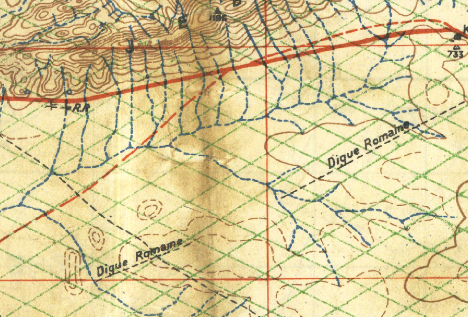
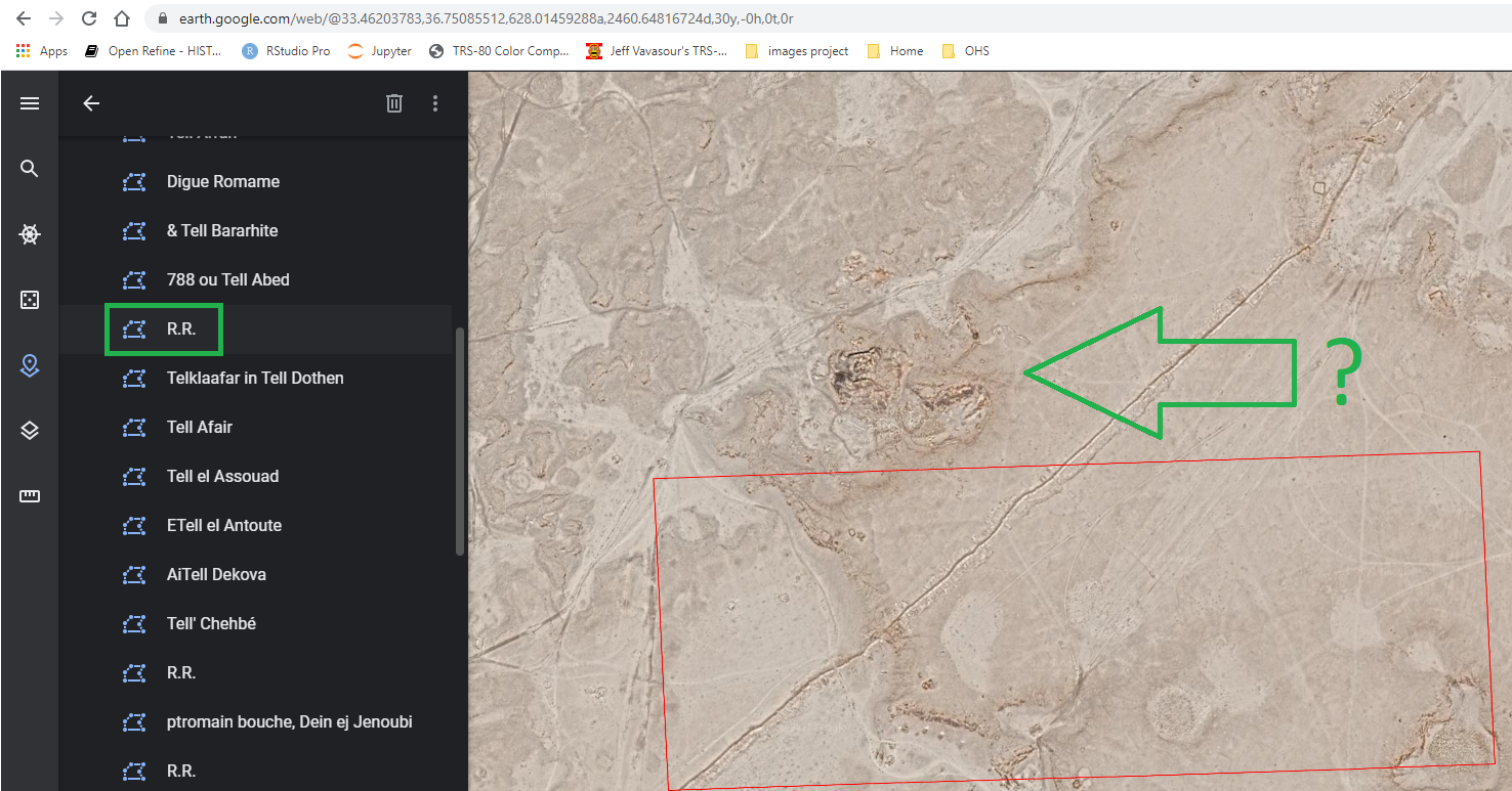
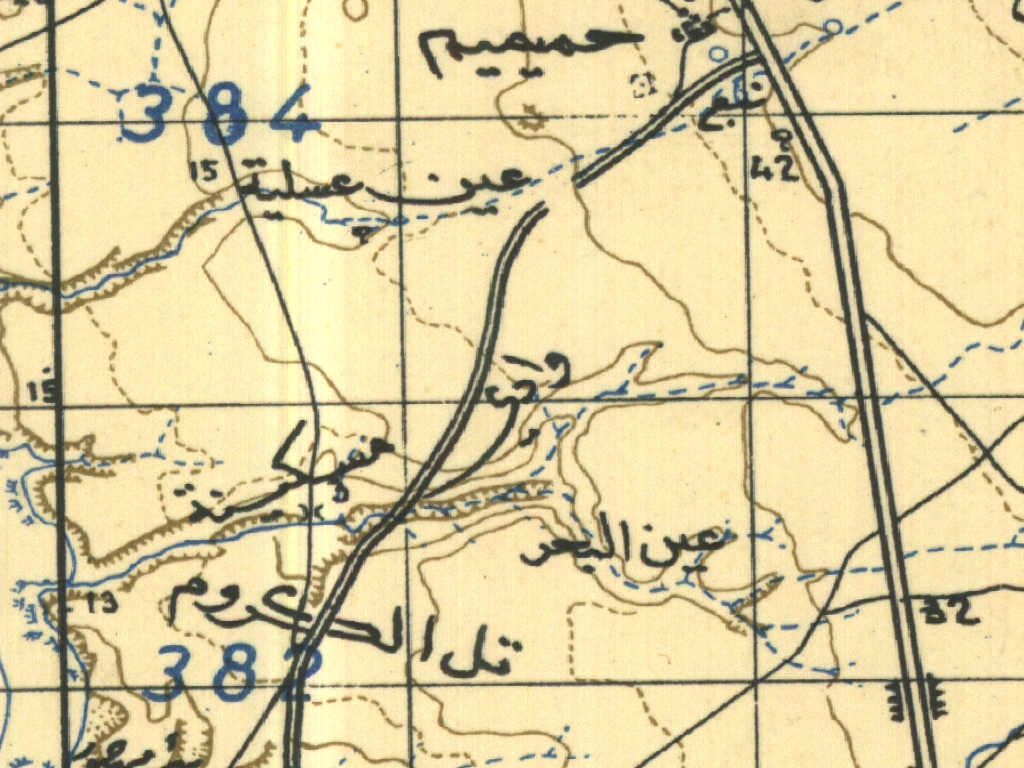
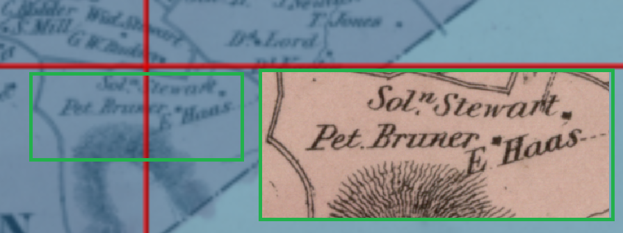
Handwriting transcription is relatively new, but is mainstream and works well. For example, see Simon Willison’s blog. The Antioch fieldbooks offer an additional challenge for transcription, they are written in pencil which does not contrast well with the background color of paper. See the image below:

At first, when I used Azure Cognitive Services to transcribe text, the results were rather poor, as per below:

1 Juin.
C'st un terrain situe a l' Est on la Renti ; inst contyn
Le pek voyia à & maism ro'sine a fm muriau
À la rent , pos ihr con Na Ih tivain - Jun 10m x3m

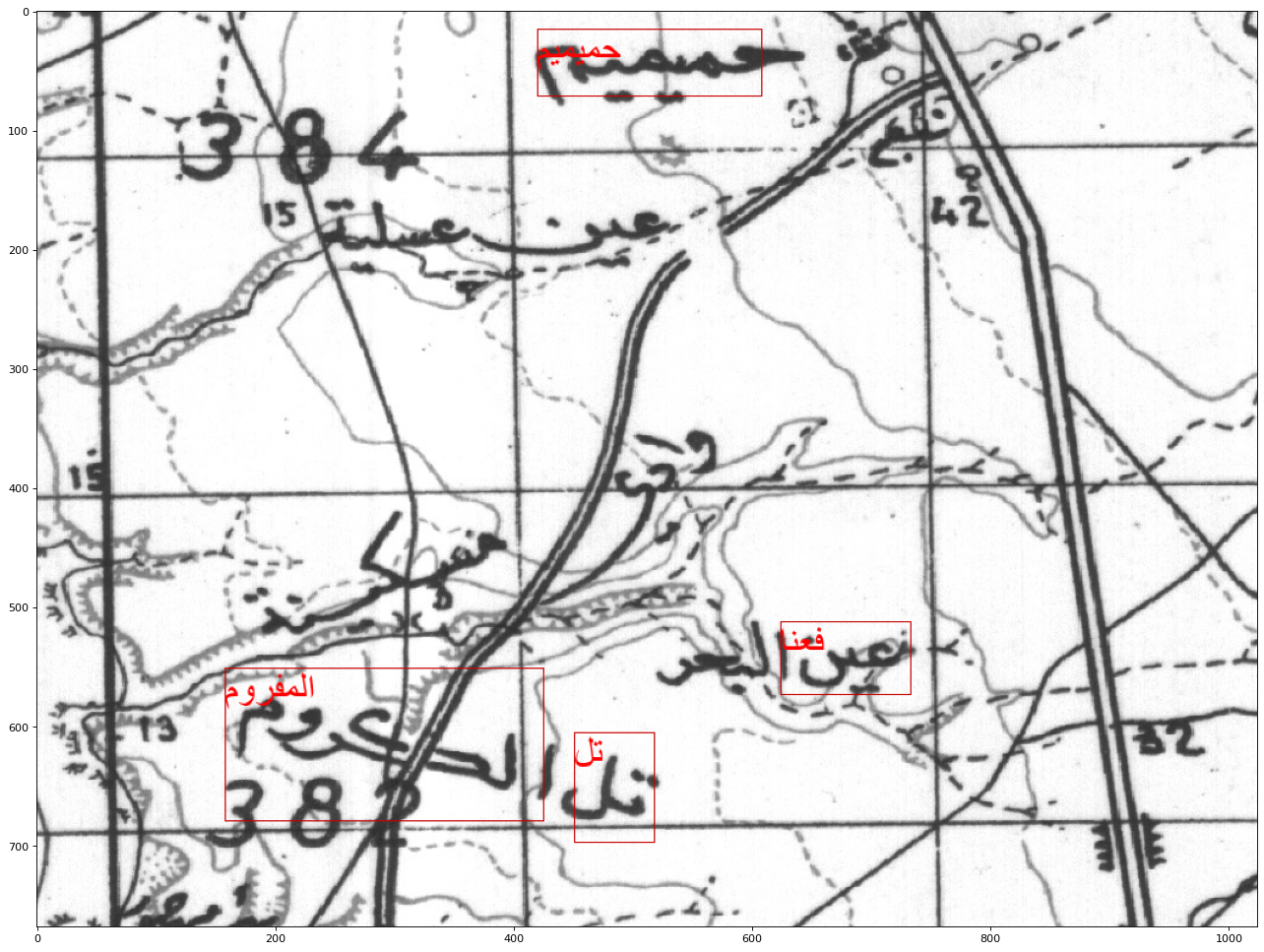
I rendered the images into black and white to increase the contrast. (Working code is here.) Below is a sample image and results.

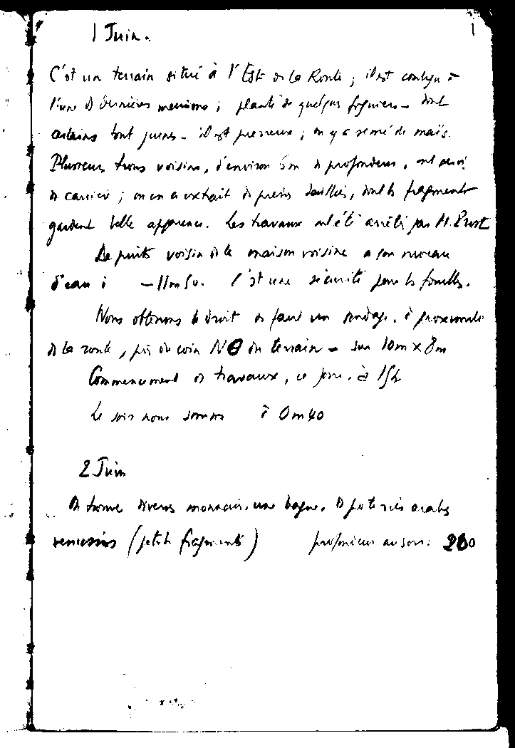
1 Juin.
C'est un terrain situé à l'Est or la Route ; il est conlyn
l'un 1 derrières massimo ; plante de quelpas figuiers - dal
acting but jeers . it off presseurs ; in ya reme'de mai's.
Plusieurs tuns voision, d'environ 5m de profondeur, as servi
À carrier ; men a extrait is press dailles, with fragment
gardent belle apparence. Les travaux net avéli pas 11. Pust
De puits voisin A la maison voisine . for nouveau
Sean : - 11mbo . I st use seemite love to fouls .
None offirms & droit as faul un povagy, è prosimale
À la conte , pi du coin NO in terrain - sun 10m xIm
Commencement 1 travaux, 4 por, à Ifhe
, Om40
2. Jun
A frame Divers monacies , une bagno . A foto ries orals
4.
remission ( patch fragments) profmeus au son : 200

As shown above, the results are better. I’d like to fine tune the image contrast process to improve results though.

Although the results improved, they are not that useful. I tried AWS Textract to improve results. For this page, here they are:

 ) Juin. C'st uin tanain situi a 1 Est is la Ronte ilst conlyn 1. Fun & burious menime; plants & guelpus togmen me anthoms but jurns it it preneure m y c remi'd mais Plusen two valian, jenvisor 5m A proformance and phri n carrier; men a extail is prems dailler, inth hagment gardent little appenence. he havane mit anition 11 Part L puils verying 1 a maison misine . for mean iean i - - limsu. / it use viamits from h fomells. Nons oftension i init to fani in andry. iproxemate 1 la wonte, , tris it win NO in train - in 10mx cm Commenument 1) havause, " pone. ' 15th le this home Jmm i Om40 2Jum time Avens moraan.un before. D fut in each renisms (ptob pro/mium wuson 260 ) Juin. C'st uin tanain situi a 1 Est is la Ronte ilst conlyn 1. Fun & burious menime; plants & guelpus togmen me anthoms but jurns it it preneure m y c remi'd mais Plusen two valian, jenvisor 5m A proformance and phri n carrier; men a extail is prems dailler, inth hagment gardent little appenence. he havane mit anition 11 Part L puils verying 1 a maison misine . for mean iean i - - limsu. / it use viamits from h fomells. Nons oftension i init to fani in andry. iproxemate 1 la wonte, , tris it win NO in train - in 10mx cm Commenument 1) havause, " pone. ' 15th le this home Jmm i Om40 2Jum time Avens moraan.un before. D fut in each renisms (ptob pro/mium wuson 260

AWS Textract translates more letters, but based on this one page, Azure Cognitive Services seems to better understand the French language text. AWS supports French, but I am not sure if there is a parameter to tell it to use French, like Azure Cognitive Services uses. Below is a program line for Azure Cognitive Services setting language = “fr”.

read_response = computervision_client.read(read_image_url,  raw=True, model_version="2022-01-30-preview", language = "fr")

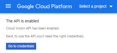
I also tried Google Cloud Platform (GCP). (I wrote about using GCP here.) GCP also supports French with “language_hints”:

    image = vision.Image(content=content)
    response = client.text_detection(
    image=image,
    image_context={"language_hints": ["fr"]},  
     )

Below are the results for the page above:

-1 | Juina C'st un terrain situé à l'Est or La Ronti ; il est conly n l'une if Juniores mecione ; plante de quelqus figniers dink orting bout joins il y preveux ; yo semé de mais . Plusieur tous voisina , d'environ 5on à profondeus , ont pris ! gardend à carrier ; men a extrait is presies desitlers , wind to fragmento belle apparence . Les travaux atét anéli par 11. Pust te punts voisin is la maison voisine a for mureau -11m Su- / sture sécurité pour to fouilles . anday presente Nons oftenons uit os fami de la conte , fis in coin NO in terrain - fon 10m x 8m Commencement of travaux , ce jour , an Ist > Omko de Join home from 2. Jum tarme Divers monnaies , un reniesios ( jetch faforint ) m * bojne foteries orals . proponicur ausen : 200 

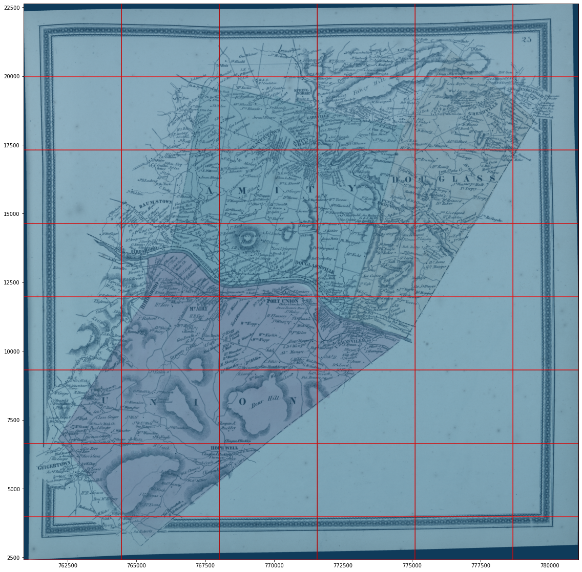
Here are some additional results for you to judge: see this page and click the “next” link to browse further. This spreadsheet lists the pages and transcribed text in the “contrasted_pages” tab.

Our project to detect relict charcoal hearths (RCHs) relies on using LiDAR data that shows the what remains of these hearths on the surface of the land. These hearths were constructed in forested areas near the trees that were felled to build them. As forests regrew, remains of RCHs were often preserved. The distinctive flat, 10-15m circular areas are visible in slope images derived from LiDAR data. Not all of these objects in forested areas are RCHs, but in Pennsylvania, many are. The density of RCHs in parts of the state is due to the extent of historical charcoal making to fuel the early steel industry. This was before steel making transitioned to using mineral coal starting in the mid-nineteenth century and completing in 1945.

In non-forested areas it is much less likely that similar looking objects are RCHs. The surfaces of non-forested areas today are more likely to be disturbed by development or agriculture since the era of charcoal making. Thus, any evidence of an RCH, even if once present, is likely to have been plowed or bulldozed over.

Given this premise, when detecting RCH it is more efficient to spend effort only on searching forested areas. At the same time, by ignoring detected objects that look like RCHs in non-forested areas, high likelihood false positive RCH detections can be removed from consideration. For these reasons, I wanted to have a vector layer of forested areas of Pennsylvania. Creating the vector layer takes several steps, described below.

PAMAP Program Land Cover for Pennsylvania, 2005

I based the forest vector layer on the PAMAP Program Land Cover for Pennsylvania, 2005. https://www.pasda.psu.edu/uci/DataSummary.aspx?dataset=1100. This is a detailed, large file size raster that describes the land cover of the state. Due to the detail, converting this entire raster file into polygons of a vector file consumed too many resources for QGIS to complete this on my machine. To solve that problem, I clipped the dataset into a smaller geographic area and then filtered the results to just forest land cover.

Clip by extent

Our project is conducting a search of RCHs in the entire state of Pennsylvania. To break the project down into smaller steps, the project searches the state by Forest District. Presently, we are searching Forest District 17 in the south east part of the state. Below is a screen shot of the land cover raster in gray scale and Forest District 17 outlined in green. The Forest District file is filtered on “DistrictNu” = 17 in QGIS.

Below is the detail of the QGIS command used to clip the raster. In QGIS’s menu it is: Raster | Extraction | Clip Raster by Mask Layer…

Input layer: ‘E:/a_new_orgs/carleton/pennsylvania_michaux/land_cover/palulc_05_utm18_nad83/palulc_05.tif’

Mask layer: ‘E:/a_new_orgs/carleton/pennsylvania_michaux/DCNR_BOF_Bndry_SFM201703/DCNR_BOF_Bndry_SFM201703.shp|subset=\”DistrictNu\” = 17’

Algorithm 'Clip raster by mask layer' starting…
Input parameters:
{ 'ALPHA_BAND' : False, 'CROP_TO_CUTLINE' : True, 'DATA_TYPE' : 0, 'EXTRA' : '', 'INPUT' : 'E:/a_new_orgs/carleton/pennsylvania_michaux/land_cover/palulc_05_utm18_nad83/palulc_05.tif', 'KEEP_RESOLUTION' : False, 'MASK' : 'E:/a_new_orgs/carleton/pennsylvania_michaux/DCNR_BOF_Bndry_SFM201703/DCNR_BOF_Bndry_SFM201703.shp|subset=\"DistrictNu\" = 17', 'MULTITHREADING' : False, 'NODATA' : None, 'OPTIONS' : '', 'OUTPUT' : 'TEMPORARY_OUTPUT', 'SET_RESOLUTION' : False, 'SOURCE_CRS' : QgsCoordinateReferenceSystem('EPSG:26918'), 'TARGET_CRS' : None, 'X_RESOLUTION' : None, 'Y_RESOLUTION' : None }

GDAL command:
gdalwarp -s_srs EPSG:26918 -of GTiff -cutline C:/Users/User/AppData/Local/Temp/processing_gEEUVX/081df2395865469b973df34e0f45f1e5/MASK.shp -cl MASK -crop_to_cutline E:\a_new_orgs\carleton\pennsylvania_michaux\land_cover\palulc_05_utm18_nad83\palulc_05.tif C:/Users/User/AppData/Local/Temp/processing_gEEUVX/899b60ac78354e019d9c2a2992ae4905/OUTPUT.tif
GDAL command output:
Copying raster attribute table from E:\a_new_orgs\carleton\pennsylvania_michaux\land_cover\palulc_05_utm18_nad83\palulc_05.tif to new file.

Creating output file that is 5681P x 4602L.

Processing E:\a_new_orgs\carleton\pennsylvania_michaux\land_cover\palulc_05_utm18_nad83\palulc_05.tif [1/1] : 0...10...20...30...40...50...60...70...80...90...100 - done.

Execution completed in 4.94 seconds
Results:
{'OUTPUT': 'C:/Users/User/AppData/Local/Temp/processing_gEEUVX/899b60ac78354e019d9c2a2992ae4905/OUTPUT.tif'}

Loading resulting layers
Algorithm 'Clip raster by mask layer' finished

To filter just the forest values, I referenced https://www.pasda.psu.edu/uci/FullMetadataDisplay.aspx?file=palanduse05utm18nad83.xml which shows values for

41 – Deciduous Forest
42 – Evergreen Forest
43 – Mixed Deciduous and Evergreen

QGIS’ raster calculator is used to the value of raster pixels to 1 if the land cover value is >= 41 and <= 43 (forested) using this formula:

1*("Clipped (mask)@1" >= 41 and "Clipped (mask)@1" <= 43)

Sieving out small areas of forest.

For the purposes of this project searching small areas of forest is unlikely to result in RCHs, thus searching these small areas may be a waste of time. To reduce that waste, the small forested areas are sieved from the raster.

Raster | Analysis |Sieve… Threshold of 9.

This raster has values 1 for forested and 0 for not. I only want to work with the forested data and so I wish to remove the 0 values. To do this in QGIS, right-click on the layer: Export | Save as… and specify 0,0 as No data values.

Create the vector layer

To create the vector layer from a raster in QGIS: Raster | Conversion | Polygonize… Name of field to create: “forested” gdal_polygonize.bat E:\a_new_orgs\carleton\pennsylvania_michaux\land_cover\d17_forest_cover_9july_just_1.tif C:/Users/User/AppData/Local/Temp/processing_exTjDd/2e62017e5fa3420b8dbfff6a5508356f/OUTPUT.gpkg -b 1 -f “GPKG” OUTPUT Forested

The conversion of a raster to vector layer takes a few minutes to process. However when I used the whole raster, before clipping, merging values, sieving and setting 0 = no data, making a vector layer took more than 1 hour and failed.

I am learning about Graph Databases. These are notes that may be useful to you, but caution is advised since I’m new to this.

What are Graph databases? They are a means to relate data as connected points using vertices (the points) and edges (the connections). Each vertex and edge has properties that describe it.

What flavours of Graph databases exist? I have been looking at neo4j.io and Azure Cosmos DB and I imagine there are more. This post works with Cosmos DB, Gremlin and Python.

Azure Cosmos DB

My notes are based on Quickstart: Create a graph database in Azure Cosmos DB using Python and the Azure portal. (Thank you to Manish Sharma, Sneha Gunda and Microsoft for this.) I’m also reading Graph Databases in Action –
Examples in Gremlin by Dave Bechberger and Josh Perryman.

Python & Gremlin

Python and the Gremlin api for the Cosmos DB graph database are used to manipulate data. Gremlin is part of the Apache TinkerPop framework for graph databases. I tried to use a Jupyter notebook on Google Colab, but kept getting “RuntimeError: Cannot run the event loop while another loop is running”. I used Visual Studio Code to edit and run the .py programs. I installed gremlinpython:

pip install --trusted-host=pypi.org --trusted-host=files.pythonhosted.org --user gremlinpython

Knowledge Graph of subjects in the diary of Capt. William White.

A study of the 1917 World War I diary of Canadian soldier Capt. William White yielded a lists of people, organizations and locations appearing in it. An analysis of these subjects may open more avenues for research into Capt. White’s experience in wartime France as well as his unit, No. 2 Construction. With this exercise I am seeking to build a knowledge graph of subjects in the diary.

The programs I am using are in Github and based on the Microsoft example. Errors in the programs are mine.

I set up a Graph database in Microsoft Azure for this exercise using the Quickstart noted above. I’m using the free tier of Azure pricing.

Preparing data

• Run drop.py to remove all of the data from the database and make it ready to load. The Gremlin statement is g.V().drop()
• The subjects in the diary are stored in a relational database. Each table was exported as a .csv. These files include wwper.csv, wwloc.csv, wworg.csv, wwpages.csv (which store the person, location, organization and page entities). The files wwper_x_page.csv, wwloc_x_page.csv and wworg_x_page.csv store the references between subjects, such as a person, and the diary page they appear on.
• A set of programs, like prep_data_1_people.py parse and reformat the .csv data into Gremlin statements that allow the data to be inserted into the graph database.
• Run all of the “prep_data_1” programs to prepare the data to be loaded.

Loading the database.

Load Vertices/Nodes

• Run data_load_people.py. This runs a set of statements to create Vertices such as: g.addV(‘person’).property(‘id’, ‘per0’).property(‘name’, ‘Capt. William White’).property(‘name_last’, ‘White’).property(‘about’, ‘No. 2 Construction chaplin’).property(‘partitionKey’, ‘partitionKey’)
• Run data_load_locations.py, data_load_organizations.py and data_load_pages.py. This completes the load of vertices.
• Check the results in Azure’s Data Explorer. Click “Execute Gremlin Query” and click on results to view each Vertex. At the present time Vertices are not related to each other.
• Change the graph style to display the name of the Vertex and differentiate node types by color, using the label field. (See picture below)

Load Edges

• Run data_load_per_x_page.py. This executes a set of statements to create Edges such as: g.V(‘per1’).addE(‘appears’).to(g.V(‘page3’)). Person ID=1 (Mlles Thomas) appears on page ID=3, seen here.
• Run data_load_loc_x_page.py and data_load_org_x_page.py. The completes the load of edges.
• Check the results in Data Explorer. Click “Execute Gremlin Query” and click on results to view each Vertex. You should see relationships now. (see below)

Next steps

The next steps are to model more meaningful relationships between entities. For example: soldiers in the same unit, members of a family, friends and related organizations.

Visual Studio Code, side note.

I am using Visual Studio Code for this. I had this error connecting to GitHub “SSL certificate problem: self signed certificate in certificate chain“. Matt Ferderer’s post here allowed me to fix this.

I also get this error message below. I am running VS Code on Windows. Thanks to this answer on Stack Overflow, it seems to be an error with aiohttp. I can’t fix it, but it does not prevent the scripts from completing.

Exception ignored in: <function _ProactorBasePipeTransport.__del__ at 0x000001B296E5FAF0>
Traceback (most recent call last):
  File "C:\Users\jblackad\AppData\Local\Programs\Python\Python39\lib\asyncio\proactor_events.py", line 116, in __del__
    self.close()
  File "C:\Users\jblackad\AppData\Local\Programs\Python\Python39\lib\asyncio\proactor_events.py", line 108, in close
    self._loop.call_soon(self._call_connection_lost, None)
  File "C:\Users\jblackad\AppData\Local\Programs\Python\Python39\lib\asyncio\base_events.py", line 746, in call_soon
    self._check_closed()
  File "C:\Users\jblackad\AppData\Local\Programs\Python\Python39\lib\asyncio\base_events.py", line 510, in _check_closed
    raise RuntimeError('Event loop is closed')
RuntimeError: Event loop is closed

These are notes for setting up a server and viewer for large images using International Image Interoperability Framework™ (IIIF).

IIIF allows large images to be streamed so they can be viewed more readily using an API rather than just downloading a huge image. IIIF is also an open standard meant to foster the exchange of images and their metadata.[See IIF FAQ.]

IIF needs a server to host the images and stream them, images and a viewer.

IIIF Server: Cantaloupe

I used Cantaloupe for the image server. It’s available on Reclaim Cloud. I opened an account, and selected Cantaloupe from the marketplace to install. See this note from Reclaim.

I uploaded an image called A14660_160.tif to /home/jelastic/images. When I use this URL for the image (https://node8039-env-3549969.ca.reclaim.cloud/iiif/2/A14660_160.tif/info.json) the server responds with JSON. [This URL won’t work if I have turned the server off to save hosting charges. Ping me if you’d like me to turn it on.] The JSON looks like this:

{"@context":"http://iiif.io/api/image/2/context.json","@id":"https://node8039-env-3549969.ca.reclaim.cloud/iiif/2/A14660_160.tif","protocol":"http://iiif.io/api/image","width":10805,"height":10779,"sizes":[{"width":84,"height":84},{"width":169,"height":168},{"width":338,"height":337},{"width":675,"height":674},{"width":1351,"height":1347},{"width":2701,"height":2695},{"width":5403,"height":5390}],"tiles":[{"width":512,"height":512,"scaleFactors":[1,2,4,8,16,32,64,128]}],"profile":["http://iiif.io/api/image/2/level2.json",{"formats":["jpg","tif","gif","png"],"maxArea":100000000,"qualities":["bitonal","default","gray","color"],"supports":["regionByPx","sizeByW","sizeByWhListed","cors","regionSquare","sizeByDistortedWh","canonicalLinkHeader","sizeByConfinedWh","sizeByPct","jsonldMediaType","regionByPct","rotationArbitrary","sizeByH","baseUriRedirect","rotationBy90s","profileLinkHeader","sizeByForcedWh","sizeByWh","mirroring"]}]}

IIIF Image Viewer

Leaflet can be used to view IIIF images. I’ve used Jack Reed’s code to view:

This GitBook is a useful resource https://iiif.github.io/training/intro-to-iiif/.

This is a note about replicating the work of Drs. Arnau Garcia‐Molsosa, Hector A. Orengo, Dan Lawrence, Graham Philip, Kristen Hopper and Cameron A. Petrie in their article Potential of deep learning segmentation for the extraction of archaeological features from historical map series. [1]

The authors demonstrate a working process to recognize map text. Their “Detector 3” targets the “word ‘Tell’ in Latin characters.” [1] As they note, “‘tell’ (Arabic for settlement mound) may appear as the name of a mound feature or a toponym in the absence of an obvious topographic feature. This convention may be due to the placement of the names on the map, or a real difference in the location of the named village and the tell site, or because the tell has been destroyed in advance of the mapping of the region.” [1]

I worked with a georeferenced map provided by Dr Kristen Hopper, Dr. Dan Lawrence and Dr. Hector Orengo: 1:200,000 Levant. Sheet NI-37-VII., Damas. 1941. The map uses Latin characters and so I used Azure Cognitive Services to transcribe the text. Below is part of the map showing “R.R.”, signifying Roman Ruins, and “Digue Romaine”, Roman dike.

This map contains a lot of text:

After transcription I applied a crude filter to remove numbers and retain places that contained lowercase text romam, roman, romai, digue, ell, r.r. Below is a sample of what was retained:

keep i :  44 Tell Hizime
keep i :  56 Nell Sbate te
keep i :  169 Well Jourdich
keep i :  182 Tell abou ech Chine
keep i :  190 ell Hajan
keep i :  221 Tell Kharno ube
keep i :  240 Deir Mar Ellaso &
keep i :  263 Dique Romam
keep i :  303 Tell Arran
keep i :  308 Digue Romame
keep i :  313 & Tell Bararhite
keep i :  314 788 ou Tell Abed
keep i :  350 R.R.
keep i :  379 Telklaafar in Tell Dothen
keep i :  388 Tell Afair
keep i :  408 Tell el Assouad
keep i :  428 ETell el Antoute
keep i :  430 AiTell Dekova
keep i :  433 Tell' Chehbé
keep i :  436 R.R.
keep i :  437 ptromain bouche, Dein ej Jenoubi
keep i :  438 R.R.
keep i :  439 Tell el Moralla!?

... etc.

Below is a screenshot of georeferenced place names displayed on a satellite image in QGIS:

The polygons containing place names are in a shapefile and kml. These locations on the map that possibly represent tells and Roman ruins. The kml can be downloaded and added to Google Earth as a Project, as shown below. This allows an examination of the landscape near each label as seen from a satellite. I have not examined these sites and I don’t have the expertise or evidence to determine whether these are archeological sites. This is meant as a proof of technology to find areas of interest. If you’d like a copy of the kml or shapefile, feel free to contact me on Twitter @jeffblackadar.

The code I used is here.

Thank you to Drs. Kristen Hopper, Dan Lawrence and Hector Orengo for providing these georeferenced maps.

[1] Garcia-Molsosa A, Orengo HA, Lawrence D, Philip G, Hopper K, Petrie CA. Potential of deep learning segmentation for the extraction of archaeological features from historical map series. Archaeological Prospection. 2021;1–13. https://doi.org/10.1002/arp.1807

As noted in an earlier post, I am working with a large set of digital maps thanks to Dr. Kristen Hopper, Dr. Dan Lawrence and Dr. Hector Orengo. As I work through these maps I want to record their attributes so I don’t need to re-open them frequently. This is a note about a process to record metadata in QGIS I am trying out.

For each map I wish to record:

• map_name.
• crs – The geographic coordinate reference system.
• extent – The coordinates of the map’s coverage.
• language – Maps are Arabic, French and English.
• year.
• color_scheme – Most maps have black text, brown topographic features and blue water features. Some maps use red and a few add green.
• ruins_symbol – Some maps use R. R. to signify a Roman Ruin. Others use a picture symbol.

For map_name I use the layer name. Crs and extent are stored as part of the geographic information in the map’s georeferenced tif.

Language can be defined in Layer Properties | Metadata.

I used Metadata Keywords to define color_scheme, ruins_symbol and year.

A small program in QGIS can export the data into a .csv.

This is the export program in QGIS:

from xml.etree import ElementTree as ETree

file_out = open("E:\\a_new_orgs\\crane\\large\\maps_syria.csv", "w")
file_out.write('"map_name","crs","extent","language","year","color_scheme","ruins_symbol"\n')

layers = qgis.utils.iface.mapCanvas().layers()
for layer in layers:
    layerType = layer.type()
    layerName = layer.name()
    if layerType == QgsMapLayer.RasterLayer:
          
        xml = QgsLayerDefinition.exportLayerDefinitionLayers([layer], QgsReadWriteContext()).toString()
        xml_root =  ETree.fromstring(xml)
        
        keywords = {'color_scheme': '', 'year': '', 'ruins_symbol': ''}
        for obj in xml_root.findall('./maplayers/maplayer/resourceMetadata'):
            print(obj)
            map_language = obj.find('language').text
            for keywords_obj in obj.findall('./keywords'):
                keywords[keywords_obj.attrib['vocabulary']] = keywords_obj.find('keyword').text
        print(keywords)
        print(str(layer.name()), layer.crs(), layer.extent())
        file_out.write('"' + str(layer.name()) + '","' + str(layer.crs()) + '","' + str(layer.extent()) + '","' + str(map_language) + '","' +str(keywords['year']) + '","' + keywords['color_scheme']  + '","' + keywords['ruins_symbol'] + '"\n' )

file_out.close()

This map below conveys a lot of information using color. Topographic lines are brown, water features are blue. It’s a visually complex map. I wanted to see if I removed non-text blue and brown features on the map, could I improve optical character recognition of the text in black. This is a quick note about the process.

I used this short program to filter the color so that features in black were retained while lighter colors were changed to white (255,255,255).

import cv2
import numpy as np
# This is the 1 map tile we'll use for this example:
from google.colab.patches import cv2_imshow
img = cv2.imread('/content/drive/MyDrive/crane_maps_syria/maps_large/Djeble_georef/jpg_tiles/r07c09.jpg',-1)
print("before")
cv2_imshow(img)

# Thanks to https://stackoverflow.com/questions/50210304/i-want-to-change-the-colors-in-image-with-python-from-specific-color-range-to-an
hsv=cv2.cvtColor(img,cv2.COLOR_BGR2HSV)

# Define lower and uppper limits of what we call "black"
color_lo=np.array([0,0,0])
color_hi=np.array([90,90,115])

# Mask image to only select black text
mask=cv2.inRange(hsv,color_lo,color_hi)

img[mask==0]=(255,255,255)

cv2.imwrite("result.png",img)
img2 = cv2.imread('result.png',-1)

print("after")
cv2_imshow(img2)

Below is the result of transcription and there is no visible benefit here. However this appears to be a useful method for separating analysis of map elements using color.

I would like to work with Arabic language maps and this post sets up transcription of one map tile using Google Cloud Vision.

I am grateful to Dr Kristen Hopper and Dr. Dan Lawrence of Durham University and Dr. Hector Orengo of the University of Cambridge for sending me a set of georeferenced digital maps to work with. Thank you!

I’m working with a map titled Djeble, dated 1942 which is centered on Jableh, Syria.

Set up Google Cloud Vision

The steps to step up the project for Google Cloud Vision are in here. https://cloud.google.com/vision/docs/setup. I have repeated the information below based on the steps I took in case it’s useful. Skip to the next step if you followed all of the instructions in the setup.

In the Dashboard of Google Cloud Platform:

Create Project and give it a name.

Check that Billing is enabled.

Enable the API.

Download the credentials as a .json. Upload the .json file to a secure directory on Google drive separate from your code. Keep this private.

Results

The program I used to do this is here: https://github.com/jeffblackadar/CRANE-CCAD-maps/blob/main/maps_ocr_google_cloud_vision_1_tile.ipynb

The above has errors and some transcriptions are missing. Still, this looks promising.

Notes about the program

In Google Colab I need to install google-cloud-vision to transcribe text and the other 3 packages to plot Arabic text.

!pip install --upgrade google-cloud-vision
!pip install arabic_reshaper
!pip install bidi
!pip install python-bidi

To transcribe Arabic text, Cloud Vision uses language_hints = “ar”. See https://cloud.google.com/vision/docs/languages.

    client = vision.ImageAnnotatorClient()

    with io.open(path, 'rb') as image_file:
        content = image_file.read()

    image = vision.Image(content=content)
    response = client.text_detection(
    image=image,
    image_context={"language_hints": ["ar"]},  
     )

To plot Arabic text, I used a font and the code below. Thanks to Stack Overflow. https://stackoverflow.com/questions/59896297/how-to-draw-arabic-text-on-the-image-using-cv2-puttextcorrectly-pythonopenc

fontpath = "/content/drive/MyDrive/crane_font/arial.ttf" # <== https://www.freefontspro.com/14454/arial.ttf  
font_pil = ImageFont.truetype(fontpath, 32)

img_pil = Image.fromarray(img)
draw = ImageDraw.Draw(img_pil)

for l in lines_of_text:
    print(l[0])
    pts = l[1]
    #This is needed to handle the Arabic text
    reshaped_text = arabic_reshaper.reshape(l[0])
    bidi_text = get_display(reshaped_text)
    draw.text((int(pts[0]), int(pts[1])),bidi_text, font = font_pil,fill=(255,0,0,255))

The next steps are process all of the tiles on the map. I also intend to process the tiles to remove some of the non-text elements on the map that confuse transcription.

The first map I transcribed using Azure Cognitive Services in a previous post was fairly small in size. As mentioned in the post about tiling, Azure Cognitive Services has limits. I’m using the free tier which accepts files up to 4mb in size. A map I am working with is 90mb, so it needs to be divided into tiles smaller than 4mb, like below.

Some of the map tiles have no text, so there is no point transcribing them. I manually eliminated the empty tiles.

The first time I transcribed a map, I placed the image on a website so Azure Cognitive Services could reference it as a URL. With the tiles, it’s easier to process them as local files and pass them to Azure. The program opens each tile as an image and sends it to Azure Cognitive Services with the computervision_client.read_in_stream() method.

def recognize_text_in_local_image(local_image_handwritten_path):
    local_image_handwritten = open(local_image_handwritten_path, "rb")
    # Call API with image and raw response (allows you to get the operation location)
    recognize_handwriting_results = computervision_client.read_in_stream(local_image_handwritten, raw=True)

The text in the tiles is transcribed and can be placed geographically.

The trouble with tiles.

Tiling is process that cuts both ways, it divides the map into smaller pieces that can be processed but it also cuts up the text. Below is part of the map (row 5, columns 2 and 3.) The names Sol.n Stewart and Pet Bruner are split over two images

Sol.n Stewart is transcribed as 2 different names: “Soln” and “tewart”. Pet. Bruner loses the er of his last name:

Overlapping the tiles solves this so that each name is displayed fully on at least 1 tile. The Tile_tiff class has a means to overlap:

tt = Tile_tiff('/content/drive/MyDrive/MaskCNNhearths/HopewellFurnace/UnionTshp_BerckCtyAtlas_1860_georef.tif',
               '/content/drive/MyDrive/MaskCNNhearths/HopewellFurnaceMapWork/tif_tiles')
tt.tt_tile_pixel_width_overlap = 200
tt.tt_tile_pixel_height_overlap = 100

tt.create_tile_files()

With the tiling, Sol.n Stewart regains a full name. Pet Bruner’s name is also made whole but gains the E. from E. Haas. However, where tiles overlap, such as on the right, there is duplication. A. Lord’s name at the bottom right is fully duplicated while T. Jones has a second version “T. Jon”.

Let’s get rid of these duplicates, but not lose useful names.

To find duplicates, the program compares all of the polygons containing text to others using: intersect_poly = poly1.intersection(poly2)

If the polygons don’t intersect, an empty polygon is returned and we know the 2 polygons are not duplicates.

If the polygons do intersect, it’s a question of how much they overlap. I assume that the smaller polygon is the one to discard if they do intersect. Some polygons will intersect that are not duplicates. The program checks to discard only smaller polygons covered 80% or more by a larger intersecting polygon. Below is the code to remove the duplicates followed by some edited output.

glist = line_text_df['geometry']
tlist = line_text_df['text']
rows_to_remove = []
print(len(glist))
for i in range(len(glist)):
    for j in range(i + 1, len(glist)):
        intersect_poly = glist[i].intersection(glist[j])

        if(not intersect_poly.is_empty):
            if(glist[i].area < glist[j].area):
                # glist[i] is smaller
                if(intersect_poly.area/glist[i].area >.8):
                    print("remove i : ", i, j, "{:3.2%}".format(intersect_poly.area/glist[i].area), int(intersect_poly.area), " Remove: ", tlist[i], int(glist[i].area), " Keep: ", tlist[j], int(glist[j].area))
                    rows_to_remove.append(i)
            else:
                if(glist[i].area >= glist[j].area):  
                    if(intersect_poly.area/glist[j].area >.8):
                        print("remove j : ", i, j, "{:3.2%}".format(intersect_poly.area/glist[j].area), int(intersect_poly.area), " Keep: ", tlist[i], int(glist[i].area),  " Remove: ", tlist[j], int(glist[j].area))
                        rows_to_remove.append(j)

Intersection coverage: 97.55% Keep: “Wag. stop” area: 131287. Remove: “Wag. stop” area: 130344.

Intersection coverage: 100.00% Remove: “T. Jon” area: 87115. Keep: “T. Jones” area: 128244.

Results:

Below is a close up of text polygons after duplicates are removed. There is only one T. Jones and Wag. Stop which is good. Although the Haas box at the bottom intersects with “Pet. Bruner E.”, it’s not removed as duplicate, which is also good. It’s too bad there is a transcription recognition error here due to word alignment and 2 nearby houses marked on the map.

Here is the resulting map:

The program to tile the maps is here. The program to transcribe the tiles and remove duplicates is here.

Sometimes geotiffs are too large to process. For example, to transcribe text on a map, as the previous post describes, Azure Cognitive Services has a size limit of 4mb for the free tier and 50 mb for the paid. Also, for deep learning related tasks, I have found it easier to divide large geotiffs into smaller, uniform size images for training and object detection.

These are notes on the tiling technique I’m using to work with geotiffs the CRANE project is using to study the ancient near east.

Before going further I wanted to reference a very interesting article: Potential of deep learning segmentation for the extraction of archaeological features from historical map series. [1] The authors demonstrate a working process to recognize map text and symbols using picterra.ch. Their technique and work with maps of Syria is of particular interest for my work on the CRANE-CCAD project. Thanks to Dr. Shawn Graham for sending me this.

Below is a large geotiff that has points of interest plotted in it for possible analysis using deep learning. This file is nimadata1056734636.tif. At 17.45 mb in size, 5254 pixels wide and 3477 high, it’s ungainly. The program tiles the geotiff into smaller 1024 x 768 images, as shown by the red grid below.

The tiles are stored in a directory with file names in the format rXXcYY.tif, where rows start with 0 from the top and columns also start with 0 from the left. Below is the tif tile from row 3, column 2.

These uniform geotiff tiles can be used to train a deep learning model or with Azure Cognitive Services. A copy of the tiling program is here.

Thank you to CRANE and Dr. Stephen Batiuk for these images.

Reference:

[1] Garcia-Molsosa A, Orengo HA, Lawrence D, Philip G, Hopper K, Petrie CA. Potential of deep learning segmentation for the extraction of archaeological features from historical map series. Archaeological Prospection. 2021;1–13. https://doi.org/10.1002/arp.1807